Dear pylinac community,
In our institute, we’ve been using pylinac’s Winston Lutz module for some years now. At the moment, I am updating it to the newest versions.
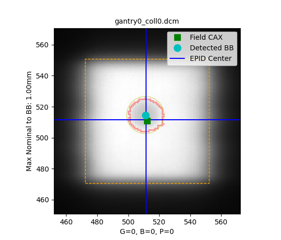
On a single image for Winston Lutz analysis, my colleagues like to also see 1) the estimated radiation field and 2) the given radius of the ball bearing. Both help us to judge if the algorithm detected the ball bearing correctly and estimate quickly the MLC movement as well.
In an older version, be solved the (1) case by using the property “rad_field_bounding_box” of the WLimage which I believe originated from a former version of the find_field_centroid function. I cannot find this funtionality anymore.
Any hints on how to access the radiation field size? At best, per individual wl image, I would plot the true radiation field as a rectangle, give the height and width, and plot the intended ideal radiation field as rectangle on top (this point I solved, as you can see in the MWE).
If anyway possible, I would like to plot the images from wl.images[…] and avoid taking the detour via wl2d. (Because: As I understood, using wl2d, I would perform an individual analysis of the given image. However, in my visualization I want to use the exact same images/results as in the 3d analysis with WinstonLutz(dir). To formulate this even clearer: I only want to plot single images. I do not want to analyze them.)
Side note: If anyone knows in which line of the source code the BB’s outline is plotted (in red), please let me know - I would like to get rid of it but could not even find the line where is it drawn.
Best regards from Munich!
Catrin
---------------------- Minimal working example ----------------------------------------
from pylinac import WinstonLutz
from pylinac.winston_lutz import Axis
from pylinac.core.image_generator import (
    GaussianFilterLayer,
    FilteredFieldLayer,
    AS1200Image,
    RandomNoiseLayer,
    generate_winstonlutz,
)

import matplotlib.pyplot as plt
import pdb

#-------------- Input -------------------------
my_dir = "wl"

#known diameter ball bearing and field size
given_bb_diam = 6
given_ideal_field_size_mm = 20

#-------------- generate demo images ----------
generate_winstonlutz(
    AS1200Image(1000),
    FilteredFieldLayer,
    dir_out=my_dir,
    final_layers=[GaussianFilterLayer(),],
    bb_size_mm=given_bb_diam,
    field_size_mm=(given_ideal_field_size_mm, given_ideal_field_size_mm),
)

#---------------- Analysis  ---------------
# Winston Lutz
wl = WinstonLutz(my_dir)
wl.analyze(bb_size_mm = given_bb_diam)
dd_results = wl.results_data(as_dict = True)

#information of a single image, here image0:
field_cax_im0 = dd_results['image_details'][0]['field_cax']
#returns a dict {'x': ... , 'y': ... , 'z': ... } in image space!

bb_location_im0 = dd_results['image_details'][0]['bb_location']
#returns a dict {'x': ... , 'y': ... , 'z': ... } in image space!

dpmm_im0 = wl.images[0].dpmm

#translating field size from coordinate mm space to image space:
given_ideal_field_size_dt = given_ideal_field_size_mm*dpmm_im0


#---------------- Visualization  ---------------
#standard Visualization
wl.plot_images()

#Visualization single image (but build from wl. not wl2d)
fig1,ax = plt.subplots()
wl.images[0].plot(ax = ax, show=False) #plain. no other information
# draw radius of given sphere diameter:
bbCircle = plt.Circle((bb_location_im0['x'], bb_location_im0['y']),
                      given_bb_diam*dpmm_im0/2, color='y', linewidth=0.5,  fill=False, label = "BB given radius")
ax.add_artist(bbCircle)
# draw the rectangle of the given field-size:
idealField = plt.Rectangle((field_cax_im0['x']-(given_ideal_field_size_dt)/2, field_cax_im0['y']-(given_ideal_field_size_dt)/2),
                          given_ideal_field_size_dt, given_ideal_field_size_dt, color="orange", linestyle='--', fill=False,
                        label="Ideal field"
)
#    ax.add_artist(idealField)
ax.add_patch(idealField)

#plot the computed field size:
# field_size_x_dt = HERE IS WHERE I NEED YOU HELP <3
# fiel_size_y_dt = HERE IS WHERE I NEED YOU HELP <3
#radField = plt.Rectangle((field_cax_im0['x']-(field_size_x_dt)/2, field_cax_im0['y']-(fiel_size_y_dt)/2),
#                          field_size_x_dt, fiel_size_y_dt, color="red", linestyle='--', fill=False,
#                        label="Computed Rad Field"
#ax.add_patch(radField)

fig1.show()