I’m trying to incorporate a leaf speed test without adding an extra field. My thought is to use the picket fence test, that way you can do the picket analysis and at the same time grab the log file associated with the picket without any extra effort. The goal is to calculate an average leaf speed value from the picket fence without regard to direction of travel. I’m using pylinac function get_snapshot_values to return both banks of leaves and their actual position. This information goes into a DataFrame using pandas where a nested for loop iterates through to obtain each leaf and its associated snapshot value. Conditional statements are also set up to help determine when the leaves have stopped and when they have started moving. The idea is to take the difference in the starting position and ending position to yield the distance traveled, count how many snapshots it took to get from starting to ending and multiply by how often the snapshots are taken (20ms for trajectory and 50ms for dyanlog) to yield time and convert to seconds, then divide distance by time and average since this is a picket fence. What I’m finding is that the leaf speed exceeds the 2.5cm/s. All positions and time were verified by looking at the csv file created for the picket and comparing those numbers with the programs numbers. Is there something I am missing or not taking into account? Any suggestions would be helpful.
Is the 2.5 cm/s defined at the isocenter or at the leaf bank?
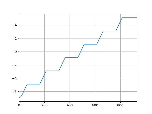
Lot going on with your algorithm so it’s hard to comment. I plotted a PF delivery (the standard Varian plan) for a leaf, plot attached. If you do a quick and dirty calc of rise/run to get travel speed between pickets it’s around 2cm/s. You could plot the leaf actual just as I did for a single leaf to get an idea of what to expect here as a sanity check for your algorithm.
log.axis_data.mlc.leaf_axes[40].plot_actual() # use whatever valid leaf number
Given that the CSV (is this a dynalog or export from pylinac?) agrees with pylinac then I’d guess it’s something to do with your algorithm for detecting start/stop motion.
Denis also has a point if you’re using raw dynalogs which needs correction for the scaling; pylinac will do this automatically (see here). Trajectory logs are defined in the iso plane normal to the beam by default.

Thank you both for the responses.
The CSV file is from pylinac using the to_csv function. The algorithm positions and time were verified with the created CSV. Within the code I have it print out what it see’s as a start position and end position, I then look at the CSV file to make sure the values are correct and they are, same with the time. If I take the difference of the starting and ending positions in the CSV, count how many snapshots it took and convert to seconds a hand calc also shows the same as the program.
I understand the Dynalogs need to be scaled and it was my understanding that pylinac already accounts for this so there is no need to input a scaling factor within the code. The snippet of code in pyliac for dynalog conversion under the from_dlog function appears to already correct expected and actual positions. Do I still need to input a scaling factor?
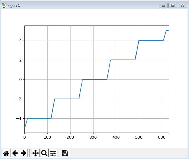
I did run an analysis on one leaf and made a plot. What are the units for the plot?

Cm and snapshots
I am not that familiar with Varian linacs, but isn’t 2.5 cm/s the max physical speed of the leaves. So at the isocenter you should get more, something like 4 cm/s?
2.5cm/s I believe is the max physical speed of the leaves. For the Dynalig files the scaling factor I believe is already taken into account within the pylinac code. I attached the actual values of the leaf positions in a csv file for viewing pleasure.
snapshot_2100CD_Daily.csv (574 KB)
Clearly a jump in position from snapshot 59-60 that isn’t physically possible; guessing the beam was off between those snapshots. See what you get when you include the beam off regions (https://pylinac.readthedocs.io/en/latest/log_analyzer.html#pylinac.log_analyzer.load_log):
log=pylinac.load_log(..., excude_beam_off=False)
I appreciate the help!! I tried your suggestion about the inclusion of the beam off regions. I believe the file I uploaded included the beam on and beam off regions. My interpretation of the file is that the repeated leaf position values are when the leaves have reached their control point and the beam is on. The other position values are when the beam is off and the leaves are moving to their next control point. If I’m wrong on that please let me know.
I tried the exclude_beam_off = False and exclude_beam_off = True. Both CSV files produced the same result, including beam on and offs.
This is what I typed:
logs = load_log(file_or_dir = “file location”, exclude_beam_off = False)
I also went back to inspect snapshot 59 and 60, but that is when the leaves have reached a control point and beam is on. Again this is how I interpret the file. There is a big change that occurs for leave 59 and leave 60 with positions at 5.06281 and -4.97433 respectively. I believe this is from going from Bank A to Bank B.
If my full code would be helpful to inspect, please let me know. I’m all for trying to figure this thing out even taking into account the scaling factor. I am told by the engineers that the C-Series software will drive the motors as fast as they will move at 100% which can exceed the 2.5cm/s. I’m just not sure how feasible 4cm/s seems.
Thanks Again!!!
I’m also interested in leaf speed as derived from log files. Initially to run from just picket fence but technically, if the code was completely automated - it could potentially check every fraction of a MLC delivery (against a QA measurement perhaps?)
Not as interested in the “actual speed” at iso - but to inspect speed constancy as it could potentially detect a “slow leaf” for delivery/treatment as part of monthly QA (or routine if its automated).
Devil’s advocate: Although, probably unlikely as encoder probably goes before motor itself (this based on rumor).
I’ve seen a eposter on aapm from July 2020 “Automated Imaging and MLC QA with Pylinac” discuss mlc speed and gantry speed QA test, but it didn’t go into details on how it was implemented.
This site on the right bottom column discusses a slow leaf detection example and has a matlab velocity algorithm, which I’m looking at:
https://www.wienkav.at/kav/kfj/91033454/physik/dmlc/dmlc_ml.htm
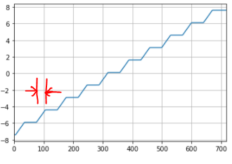
For Picket Fence MLC speed analysis - I’m thinking to measure leaf speed between pickets:
Red bars are the times between pickets.
To find a slow leaf, assuming easiest to create a “baseline” trajectory log and a test case trajectory log and inspect any atypical ratios for speed constancy changes.
I’m currently looking at the CSV files generated from log analysis and initially approach transit time calc using the actual leaf position - when it starts moving from a constant position to when it stops moving.
Welcome any thoughts - if this wheel has already been invented. Thanks.


I appreciate the help!! I tried your suggestion about the inclusion of the beam off regions. I believe the file I uploaded included the beam on and beam off regions. My interpretation of the file is that the repeated leaf position values are when the leaves have reached their control point and the beam is on. The other position values are when the beam is off and the leaves are moving to their next control point. If I’m wrong on that please let me know.
I tried the exclude_beam_off = False and exclude_beam_off = True. Both CSV files produced the same result, including beam on and offs.
This is what I typed:
logs = load_log(file_or_dir = “file location”, exclude_beam_off = False)
I also went back to inspect snapshot 59 and 60, but that is when the leaves have reached a control point and beam is on. Again this is how I interpret the file. There is a big change that occurs for leave 59 and leave 60 with positions at 5.06281 and -4.97433 respectively. I believe this is from going from Bank A to Bank B.
If my full code would be helpful to inspect, please let me know. I’m all for trying to figure this thing out even taking into account the scaling factor. I am told by the engineers that the C-Series software will drive the motors as fast as they will move at 100% which can exceed the 2.5cm/s. I’m just not sure how feasible 4cm/s seems.
Thanks Again!!!
Clearly a jump in position from snapshot 59-60 that isn’t physically possible; guessing the beam was off between those snapshots. See what you get when you include the beam off regions (https://pylinac.readthedocs.io/en/latest/log_analyzer.html#pylinac.log_analyzer.load_log):
log=pylinac.load_log(…, excude_beam_off=False)
2.5cm/s I believe is the max physical speed of the leaves. For the Dynalig files the scaling factor I believe is already taken into account within the pylinac code. I attached the actual values of the leaf positions in a csv file for viewing pleasure.
I am not that familiar with Varian linacs, but isn’t 2.5 cm/s the max physical speed of the leaves. So at the isocenter you should get more, something like 4 cm/s?